Factors influencing Google My Business listing rankings: an exploratory statistical analysis
- Factors influencing Google My Business listing rankings: an exploratory statistical analysis
- Abstract
- Introduction
- Methodology
- Results, Part 1: Global criteria and trends influencing position
- Results, Part 2: Local rotation mechanism
- Analysis and discussion
- Operational implications
- Open conclusion
- Appendix 1: Local observation vs. global trend
- Appendix 2: Linearity breakdown past position 50
Abstract
This study explores the ranking mechanisms of Google My Business / Google Business Profile listings and the factors influencing their position in Google Maps, the Local Pack, and the "Places" tab. It attempts to distinguish solid leads from noise for further investigation.
The analysis relies on two complementary approaches:
- A global study, seeking to identify the influence of various listing characteristics on their ranking using statistical models, primarily linear regression.
- A dynamic analysis, examining ranking fluctuations throughout the day and revealing a rotation phenomenon that remains largely undocumented.
The goal is to identify mechanisms that explain or describe the behavior of the algorithm responsible for establishing the hierarchy of results on Google Maps, as well as on equivalent surfaces such as the Local Pack and the "Places" tab of the SERP. A better understanding of the Google Maps algorithm would allow businesses to better leverage a channel that, in local digital marketing, proves to be particularly effective at generating qualified leads at near-zero cost.
Introduction
While it is obvious that local search ranking plays a determining role in a local business's ability to attract new customers and generate revenue, the opacity of algorithms developed by platforms like Google and Meta maintains a certain confusion. This lack of understanding fosters the emergence of myths and questionable beliefs.
A great deal of information circulates about the criteria taken into account by the Google Maps algorithm. However, it often suffers from a lack of transparency (Google mentions certain concepts but without truly defining them) or from an overly contextual and specific approach: case studies, anecdotes from professionals, advice thrown out without real justification. Most of the time, what passes for knowledge is really expert opinion, grounded in experience and the occasional resolution of specific problems, but rarely in a deeper analysis of the underlying mechanisms. These approaches are not without value, and the expertise of field professionals remains precious. However, they often rely on empirical observations without attempting to model the mechanisms themselves.
My goal here is not to challenge these experience-based insights, but rather to adopt a more systematic approach to identify verifiable trends and go beyond one-off observations. As a local marketing professional, it seemed essential to better understand these mechanisms and the factors influencing business listing rankings.
While several aspects of traditional SEO are well documented, such as the use of PageRank (whose mathematical workings are detailed in The PageRank Citation Ranking: Bringing Order to the Web by Larry Page & Sergey Brin), or more broadly the initial architecture of Google described in The Anatomy of a Large-Scale Hypertext Web Search Engine, these mechanisms have since evolved considerably. To date, no source provides a transparent view of them, and Google itself has made this machinery opaque by discontinuing PageRank disclosure in 2016. The major leak of March 2024, while revealing the existence of thousands of ranking attributes and re-ranking algorithms, ultimately provided little insight into their precise workings.
And even if we had complete information about traditional SEO, the object of study here is a distinct system: the ranking of Google Business Profile listings on Google Maps. A sub-discipline of search engine optimization that, to this day, has no dedicated scientific literature. It is worth noting the work done by Whitespark, which in its "Local Search Ranking Factors" studies proposes criteria by surveying SEO experts. But this approach, in my view, would benefit from a detailed publication and complementary methodologies. This paper fits into that dynamic, not in an attempt to "do better," but to provide an empirical and complementary contribution.
Hence the choice of an exploratory statistical approach: collect a dataset of business listings, analyze the data to identify global trends, but also examine the dynamics of the local system to observe and document specific phenomena.
Methodology
This section describes in detail the data collected, the samples used, and the analytical methods applied.
Part 1: Global criteria and trends influencing position
Why a global approach?
One of the main challenges of this study lies in the analysis of local data. When examining only the results of a specific query (e.g., "car rental Lyon"), it becomes difficult to identify clear trends. This difficulty is largely due to algorithmic noise: variability or unpredictable fluctuations in an algorithm's results, caused by uncontrolled or unknown factors. In the case of Google Business Profile rankings, this noise may be caused by algorithmic adjustments, result personalization, or real-time updates. The rotation mechanism presented in Part 2 appears to be the prime suspect for explaining this noise.
To overcome this constraint, I compiled the results of multiple local searches and computed the mean values of each criterion as a function of position. This approach helps reveal potential trends by dampening the noise and allows us to evaluate the relationship between different variables and listing rank. When these relationships appear linear, they can then be analyzed using regressions.
Data collection and sample construction
The sample consists of multiple local results compiled into a single dataset containing the following information:
Position: The listing's rank in the results at the time of collection. Position determines a listing's impression share and interaction rate. For the uninitiated: "position" on Google Maps is never directly communicated by Google through its reporting tools.
Informational fields: Title, description, phone number, address, postal code, number of reviews, average rating ("all-time," as opposed to the 30-day average), presence of links to Facebook and Instagram pages, booking link, latitude and longitude, number of images.
Supplementary data: A second collection was performed after the first to retrieve recent engagement indicators: number of reviews left in the last 30 days, number of reviews that received a response in that period, rating attributed to each new review.
Keyword occurrence: For each listing, I counted the presence of a query-specific keyword (e.g., profession name, city name) in the title and description.
Some data points were manipulated through simple calculations to construct additional potential explanatory variables: average rating over the last 30 days, number of completed fields, and distance from the centroid (I hypothesized that the further a listing is from the center of the Google Maps search screen, the worse its position).
Data was collected via API (to avoid potential user biases such as search history or geolocation). The queries were constructed as follows:
- 8 professions: hairdressers, osteopaths, mechanics, psychologists, car rental, opticians, heating technicians, and restaurants.
- These 8 professions were searched across the 40 most populated cities in France.
Although these cities and professions have nothing to do with each other, they were chosen to ensure a high volume of results. Each query result page is governed by its own dynamics specific to that query; each result is singular, even when comparing "plumber Lyon 1st" to "plumber Lyon 6th."
The final sample contains 33,135 listings and their respective positions, up to a maximum of 200 positions per query. As for the variables chosen, the selection was straightforward: no additional data can be extracted beyond what was collected.
Analytical method
The enriched sample was then reduced to a matrix presenting, by position, the mean values of: number of photos, total number of reviews, average rating (all-time), number of reviews in the last 30 days, number of review responses in the last 30 days, rating over the last 30 days, distance from centroid, average keyword occurrence in title, average keyword occurrence in description, and number of completed fields.
The sample was then restricted to the top 50 positions for two reasons:
- The distribution becomes uneven past position 50.
- Heteroscedasticity issues (unequal variability of residuals) affect the linearity of observed relationships.
Each data point was then treated as a potential explanatory variable (x), and I computed the coefficient of determination (R²) against position (y) in the context of a linear regression.
R² is a statistical indicator that measures the proportion of variance in the dependent variable (here, position) that is explained by one or more independent variables (here, the potential explanatory variables). It ranges from 0 to 1:
- R² close to 1: The explanatory variable predicts the dependent variable well.
- R² around 0.5: The explanatory variable is a moderate predictor.
- R² close to 0: The explanatory variable has almost no relationship with the dependent variable.
Note: in linear relationships, a high R² generally implies a strong correlation coefficient (R), since R² represents the proportion of variance explained by the model. This is why I deemed it unnecessary to report R separately.
Part 2: Local rotation mechanism
Why a local approach?
While Part 1 highlights global trends, a local approach allows us to examine specific phenomena that are more directly observable in a real-world context. By studying position evolution hour by hour on a single query, we can detect dynamics that are both invisible at the macro scale and imperceptible if the object is not observed over time. We therefore reduce the sample size but add an enriching temporal dimension.
Data collection and sample construction
Data collection followed the same method as Part 1, with the following differences:
- Data was collected for a single query ("location voiture Lyon" / "car rental Lyon").
- Collection was performed hour by hour over a single day, from 00:30 to 22:30.
The sample tracks the hourly position of 190 listings.
Analytical methods
Several derived metrics were constructed from the sample:
- Hourly position variation: Difference between position at time t and at t-1, enabling analysis of individual listing volatility.
- Hourly rotation rate: Proportion of listings that changed position at each hour, to identify periods of high instability.
- Mean daily variation: Sum or mean of variations over the day, per listing.
Results, Part 1: Global criteria and trends influencing position
This first analysis aims to identify the factors influencing Google Business Profile listing rankings. Specifically, we seek to measure the extent to which certain explanatory variables are correlated with listing position, through the coefficient of determination (R²) presented in the methodology. We are looking primarily for linear relationships.
Relationship between each explanatory variable and position
The figures below represent the relationship between position and each explanatory variable. The R² is specified for each. All data used corresponds to the methodology described above.
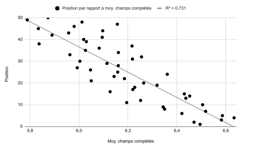
Position vs. average number of completed fields (Figure 1): A fairly strong linear trend with a substantial R² of 0.73.
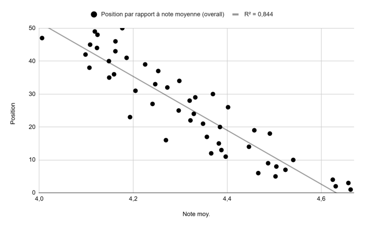
Position vs. average rating, all-time (Figure 2): A linear trend with a high R² of 0.84.
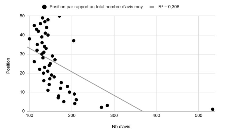
Position vs. average total number of reviews (Figure 3): A non-linear relationship with a rather low R² of 0.30. The presence of outliers is also notable (e.g., the data point at 533 average reviews for position 1). We will return to this chart in the analysis section.
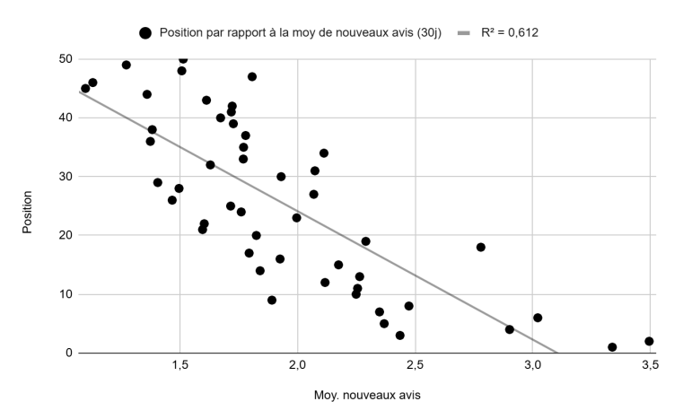
Position vs. average number of new reviews, last 30 days (Figure 4): A fairly linear relationship with a significant R² of 0.61.
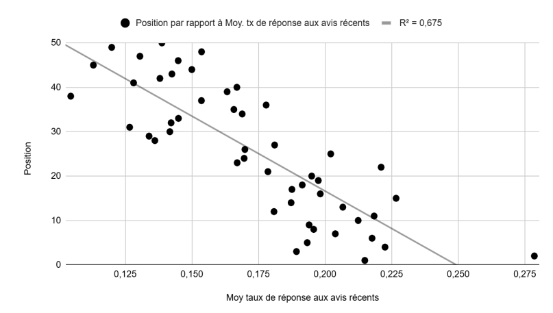
Position vs. review response rate, last 30 days (Figure 5): Response rate = (number of reviews responded to) / (number of reviews left in the last 30 days). A fairly linear relationship with a significant R² of 0.67. We will address collinearity risks in the analysis section.
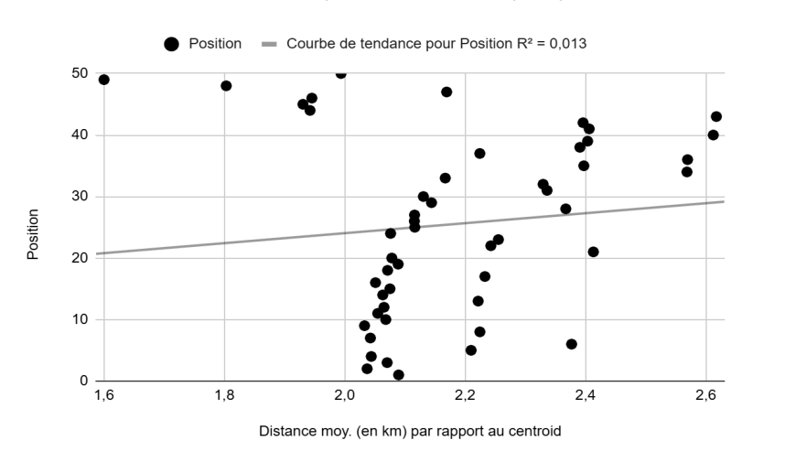
Position vs. average distance from centroid, in km (Figure 6): Absolutely no linear relationship, with a near-zero R² of 0.01.
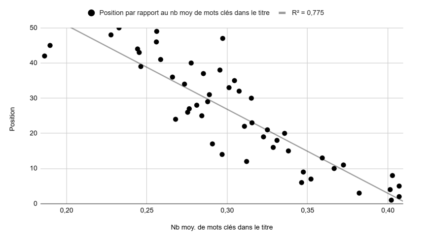
Position vs. average number of keywords in title (Figure 7): A fairly linear relationship with an R² of 0.775.
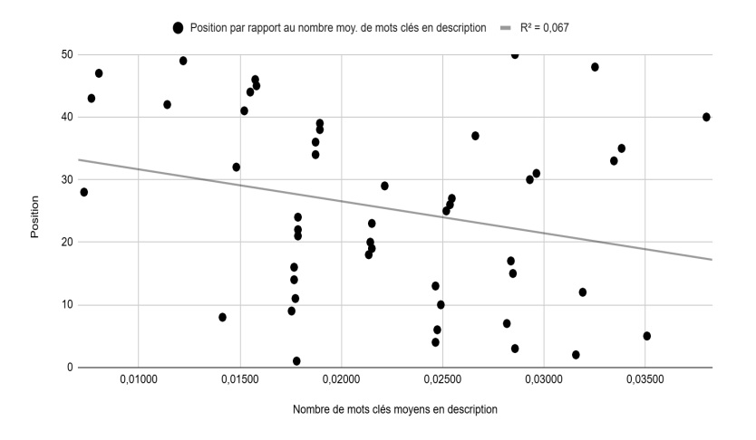
Position vs. average number of keywords in description (Figure 8): No linear relationship, with a very low R² of 0.067.
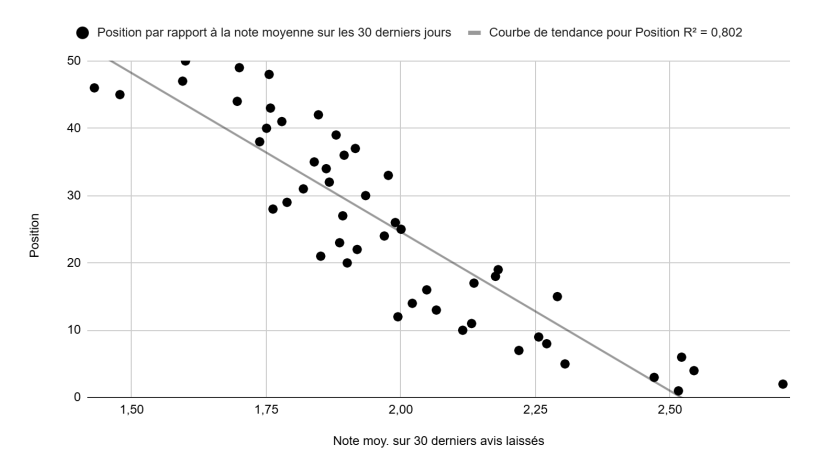
Position vs. average rating, last 30 days (Figure 9): A strong linear relationship with an R² of 0.80.
Summary of R² values
| Position relative to... | R² |
|---|---|
| Number of completed fields | 0.73 |
| Rating (all-time) | 0.84 |
| Rating (last 30 days) | 0.80 |
| Number of reviews (all-time) | 0.34 |
| Number of reviews (last 30 days) | 0.61 |
| Review response rate (last 30 days) | 0.67 |
| Number of keywords in title | 0.775 |
| Number of keywords in description | 0.067 |
| Distance from centroid | 0.013 |
| Number of photos | 0.43 |
| Multivariate linear regression (all variables above) | 0.91 |
| Adjusted R² (multivariate) | 0.90 |
Results, Part 2: Local rotation mechanism
These results were obtained by analyzing results for a single query, collected every hour of the day, as described in the methodology. I hypothesize (not formally demonstrated here) that this phenomenon is what renders the influence of the variables analyzed in Part 1 nearly imperceptible at the local level.
Position of each listing by hour of day (Figure 11)
Each line represents a single listing (Most will see an ugly figure, I see a beautiful chaos).
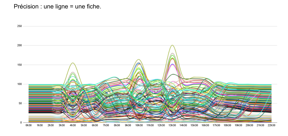
We observe:
- Two periods of low variation: between 00:30 and 02:30, and again in the late evening from 19:30 to 22:30.
- Multiple sequences with major movements: 3:30-5:30, 9:30-11:30, 12:30-14:30.
- Sequences with more moderate movements: 5:30-9:30, 11:30-12:30, 15:30-17:30.
Position appears as a dynamic variable, not a fixed data point. I call the phenomenon captured here "position rotation." Rotation is a well-known phenomenon in SEA and SEO, hence the same name. However, it is almost never mentioned in the context of Google Maps.
Variation amplitude of each listing by hour (Figure 12)
This figure makes the rotation phenomenon more visible and quantifies the amplitude of position variation for each listing at each hour of the day. The "contraction" observed at 01:30 is explained by the calculation method: the first recorded data point is the position at 00:30, and the second represents the difference between the position at 01:30 and that at 00:30. The stability of listings over this interval concentrates variations around zero.
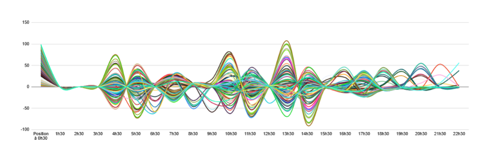
We also observe unequal movements across time slots: very restricted variations early in the morning (1:30-3:30), more moderate ones (6:30-9:30, 15:30-22:30) limited to roughly +/-50 positions, and much larger ones (4:30-5:30, 10:30-14:30).
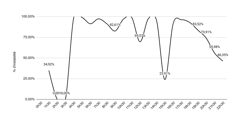
Percentage of listings changing position per hour (Figure 13)
This figure tracks the proportion of instability (% of listings whose position changes from one time slot to the next) by hour. Every single listing changed position at least once during the day.
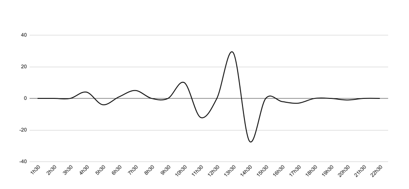
Zero-sum variations (Figure 14)
This is an extremely important observation: the variations cancel each other out. The position increase at 3:30-4:30 is immediately compensated by the one at 5:30-6:30. Sometimes this compensation is spread across two or more sequences.
| Metric | Value |
|---|---|
| Total listings | 190 |
| Listings with mean daily variation = 0 | 151 (79%) |
| Listings with mean daily variation between -5 and +2 | 39 (21%) |
The same zero-sum phenomenon holds for the overwhelming majority of listings (79%). The remaining 21% may be listings that were penalized or rewarded for a particular reason not identified here.
This means that any single-point measurement of a listing's position is unreliable. It is imperative to record positions throughout the entire day for an accurate analysis. Hourly measurements are more precise but remain an approximation.
Analysis and discussion
Critical distance from the global analysis
The results allow us to identify several interesting trends regarding the factors influencing Google Business Profile rankings. By combining all variables with a significant R² into a multivariate linear regression model, we obtain an R² of 0.91 and an adjusted R² of 0.90. This means the model explains the variance in positions reasonably well. However, in a predictive context, this model quickly reaches its limits and fails to provide precise results. The predictions of a linear regression model are only valid within the original data range. Our dataset was transformed (mean of variables by position to reduce local noise), making any extrapolation attempt illusory.
I prefer to summarize Part 1 as a practical system for eliminating suspect explanatory variables: if a variable does not maintain a linear (or polynomial) relationship with position, then there is no reason to consider it a determining factor.
Another point of caution concerns collinearity between certain variables, which can make coefficients unstable and hinder interpretation. Moreover, it is essential to remember that correlation does not imply causation: a statistical relationship between two variables does not necessarily mean a causal link.
Furthermore, the relationship between position and total number of reviews (Figure 3) is poorly evaluated here. The relationship between these two variables is not linear but rather polynomial. A linear approach is therefore ill-suited. A potential improvement would be to apply non-linear transformations to the data, such as taking the square root of position to better capture the dynamics. More precisely: the R² of 0.34 measured over positions 1-50 rises to 0.425 when restricted to positions 6-38, suggesting that the influence of review count is real but not uniform across the full range. This also means that the value of a review depends on the rating it carries. Focusing solely on volume is too reductive.
To refine the analysis and develop a more robust predictive model (though that is not the objective here), it would be more pertinent to abandon multivariate linear regression in favor of models capable of integrating categorical and temporal variables and better suited to collinearity problems.
At this stage, the global approach confirms the influence of certain variables on listing rankings, but it is not sufficient to precisely model their impact (weight or coefficient).
Critical distance from the local analysis
Due to the raw and minimally transformed nature of the collected data, the observations from this part are probably the least debatable. However, they require further validation: it seems imperative to reproduce the protocol on other queries and sectors to verify whether the same phenomena manifest. If these trends are confirmed, it would open the way to exploring hypotheses that refine our understanding of the algorithm.
The "zero-sum variations" finding (Figures 14 and 15) stands out as particularly compelling: the pattern seems too consistent to be the product of chance, as if the algorithm is expressing itself clearly here and hinting at an authentic revelation if we look more closely at the listings whose mean daily variation is not zero. What happened to them? Did one or more of the variables identified in Part 1 change? I believe that studying this subset in greater depth could reveal a great deal.
Operational implications
If the observations presented here are confirmed:
Rethink position measurement. Position should never be reduced to a single-point reading. Multiple snapshots throughout the day are necessary.
Pay much more attention to explanatory variables. A separate study conducted on over 115,000 multi-location brand listings shows that serious gaps remain in listing field completion rates and review response rates. If it turns out that these variables play a role and we can quantify their impact, it becomes immediately easier (and justified) to allocate resources to improving them.
Be careful with title keywords. While a fairly pronounced linear relationship exists between the number of keywords in the title and position (Figure 7), and while empirical observation confirms improved positioning after title optimization, the practice has been formally prohibited by Google since July 2023. While it went unsanctioned for a time, automated suspensions have increased significantly since August 2024.
Open conclusion
The Analysis and Discussion section already synthesizes the main findings. Rather than repeating a conventional conclusion, I want to open a reflection on how I believe the algorithm works. What follows is highly speculative and has not been demonstrated.
Imagine that:
-
Somewhere in the algorithm's mechanics, there exists an estimated position value. This value would be determined by the volume of searches performed for a given day and hour, as well as the expected average interaction rate for that position. Google is entirely capable of computing such metrics, and similar systems are already used by automated bidding strategies in Google Ads.
-
The variables maintaining a linear relationship (identified in Part 1) allow the algorithm to calculate a form of "primordial score" for each listing, analogous to the Quality Score in paid search or a similar mechanism in organic SEO.
-
The algorithm also takes into account each listing's declared opening and closing hours.
If these hypotheses are correct, then the algorithm's primary role would be to ensure an optimal distribution of positions by allocating to each listing an impression share (or other performance indicators such as clicks, calls, or direction requests) proportional to its primordial score. This interpretation does not contradict the observations in this study. The global analysis hints at the existence of a primordial score, while the rotation phenomenon could be explained by the need to allocate to each listing the visibility it deserves based on its score, within the constraints of its opening hours.
This approach invites us to reconsider the notion of "position," which we ordinarily imagine as quite static, and move toward something much more fluid and dynamic, a function of immediate or recent local demand. A disorienting perspective, but one that seems far more consistent with the observations of this study.
Hypotheses for future research
- Position rotation is not influenced by time slots per se, but by the overall search volume on the sector and query peaks. In a manner similar to Google Search Console in SEO, a listing's true position would in fact be the average of its positions across all impressions over a defined period.
- Listings whose sum of position variations is positive are those for which at least one of the variables identified in Part 1 was improved during the observation period.
- A listing's mean daily position is determined by a score computed from the variables identified in Part 1.
- If a listing's postal code differs from the city mentioned in the query, it automatically receives a position penalty.
- A listing flagged as "closed" at the time the query is performed automatically receives a position penalty.
- Positions are distributed as a function of both the primordial score and the listing's declared opening hours.
- The value of a given position is influenced by the historical search volume for a specific hour and day. The algorithm uses this value to assign top positions to the listings it deems most deserving.
Appendix 1: Local observation vs. global trend
To illustrate the complexity of local observation and justify the need for a global approach, consider two figures: Figure 16 shows the relationship between "average rating" and "position" at the local level (a single query: "Restaurant Grenoble"). Figure 17 shows the same relationship at the global level after the transformations described in the methodology.
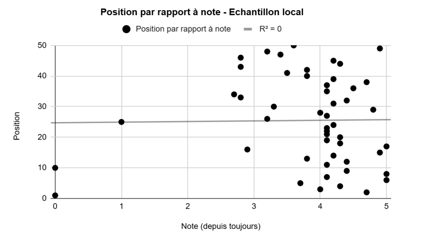
At the local level, the relationship appears completely chaotic (R² = 0), due to the rotation phenomenon observed in Part 2. At the global level, the same variables produce a clean linear trend with an R² of 0.84.
Appendix 2: Linearity breakdown past position 50
The figure below shows the variable "average number of keywords in title" (similar to Figure 7) but this time across positions 1 to 200 rather than 1 to 50. The linearity of the relationship breaks down after position 50 (R² drops to 0.028 over the full range). This is why the global study restricts the analysis to the top 50 positions.
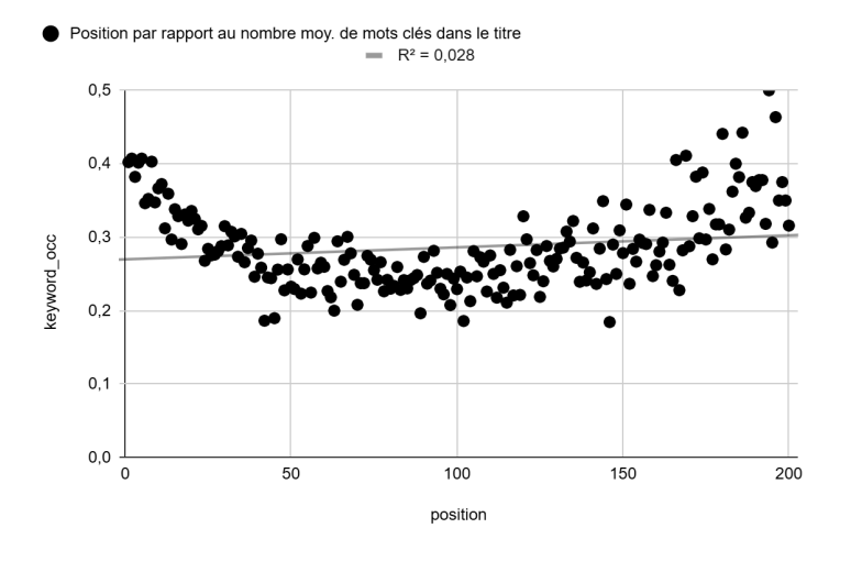
This breakdown could be explained by several hypotheses: Google may only actively compute rankings for the top listings, leaving the rest in a form of cold storage. Or the heteroscedasticity of the data past position 50 simply overwhelms any linear signal. More practically, almost nobody scrolls past the 50th result, which may mean Google simply invests less algorithmic effort in ordering those positions precisely.
Numerous alternative hypotheses and mathematical approaches could be built on this observation. It remains one of the most promising avenues for future research.